📘 Chapters covered — Topics & Cross-Refs Click to open
Fluid Mechanics — Conventions & Notation
Beginner-friendly crib sheet of symbols seen in classical fluid mechanics.
Primary source: G. K. Batchelor, An Introduction to Fluid Dynamics, Cambridge University Press, 2000.📖 Batchelor — Chapter 1 (All topics)
1) Overview
What the chapter sets up
- Continuum viewpoint: fields \( \mathbf{u}(x,t), p(x,t) \).
- Kinematics vs dynamics: strain-rate vs forces (pressure, viscous stress).
- Key measures: \( \nabla\!\cdot\!\mathbf{u} \) (dilatation), \( \boldsymbol{\omega}=\nabla\times\mathbf{u} \).
- Forces: body (gravity) & surface (stress \( \sigma_{ij} \)).
- Incompressible: \( \nabla\cdot\mathbf{u}=0 \); streamlines & potentials for irrotational parts.
Why it matters
- Sets the tensor/operator language for Navier–Stokes.
- Links vortices/streamlines to math used in BL & potential flow.
2) Subscripts & Index Notation
- \( i,j,k\in\{1,2,3\} \) label \(x_1,x_2,x_3\) (aka \(x,y,z\)); \(u_i\Rightarrow (u,v,w)\).
- Repeat index ⇒ sum. Example \(u_i u_i=|\mathbf{u}|^2\).
- \( \mathbf{a}\!\cdot\!\mathbf{b}=a_i b_i \), \( (\nabla\times\mathbf{u})_i=\varepsilon_{ijk}\partial u_k/\partial x_j \).
- \( \sigma_{ij} \) symmetric for simple fluids; traction \(t_i=\sigma_{ij}n_j\).
- \( e_{ij}=\tfrac12(\partial_i u_j+\partial_j u_i) \).
- Kronecker \( \delta_{ij} \), Levi-Civita \( \varepsilon_{ijk} \).
- Polar: \(u_r,u_\theta\); Cyl: \(u_r,u_\theta,u_z\); Sph: \(u_r,u_\theta,u_\phi\).
3) General Symbols
- Boldface vectors (e.g., u).
- \(\mathbf{x},\mathbf{x}'\); \(r=|\mathbf{x}|\); relative \(\mathbf{s}=\mathbf{x}-\mathbf{x}'\).
- Speed \(q=|\mathbf{u}|\); time \(t\).
- Material derivative \( \tfrac{D}{Dt}=\partial_t+\mathbf{u}\cdot\nabla \).
4) Coordinates & Velocity Components
| System | Coordinates | Velocity |
|---|---|---|
| Cartesian | \(x,y,z\) or \(x_1,x_2,x_3\) | \(u,v,w\) or \(u_1,u_2,u_3\) |
| Polar (2D) | \(r,\theta\) | \(u_r,u_\theta\) |
| Spherical | \(r,\theta,\phi\) | \(u_r,u_\theta,u_\phi\) |
| Cylindrical | \(r,\theta,z\) | \(u_r,u_\theta,u_z\) |
5) Flow Quantities
- Dilatation \( \Delta=\nabla\cdot\mathbf{u} \).
- Vorticity \( \boldsymbol{\omega}=\nabla\times\mathbf{u} \).
- Rate-of-strain \( e_{ij}=\tfrac12(\partial_i u_j+\partial_j u_i) \).
- Stream function \( \psi \) (2D/axisymmetric) enforces continuity.
6) Stream-Function Formulas
2D (x–y)
\( \mathbf{B}=(0,0,\psi),\quad u=\partial\psi/\partial y,\; v=-\partial\psi/\partial x \)Axisymmetric (Cylindrical \(r,\theta,z\))
\( B_\theta=\psi/r,\; u_r=\tfrac{1}{r}\partial_z\psi,\; u_z=-\tfrac{1}{r}\partial_r\psi \)Axisymmetric (Spherical \(r,\theta,\phi\))
\( B_\phi=\psi/(r\sin\theta),\; u_r=\tfrac{1}{r^2\sin\theta}\partial_\theta\psi,\; u_\theta=-\tfrac{1}{r\sin\theta}\partial_r\psi \)📖 Panton — Chapter 1 (Intro to Incompressible Flow)
Main idea: Foundation for incompressible flow — physics, assumptions, and math framework.
1.1 What is Incompressible Flow?
- Density ~ constant; often valid for Mach \(M \lesssim 0.3\).
1.2–1.4 Field Variables & Material Derivative
- \( \mathbf{u}(x,t),\,p(x,t),\,T,\,\rho,\,\mu \); Eulerian vs Lagrangian; \( \frac{D}{Dt}=\partial_t+\mathbf{u}\cdot\nabla \).
1.5–1.7 Conservation & Vorticity
- Continuity \( \nabla\cdot\mathbf{u}=0 \); momentum (leads to N–S); \( \boldsymbol{\omega}=\nabla\times\mathbf{u} \).
1.8–1.9 Streamlines & Reynolds number
- Streamlines/pathlines; \( \mathrm{Re}=\rho U L/\mu \).
Ref: Panton, Incompressible Flow, Ch. 1.
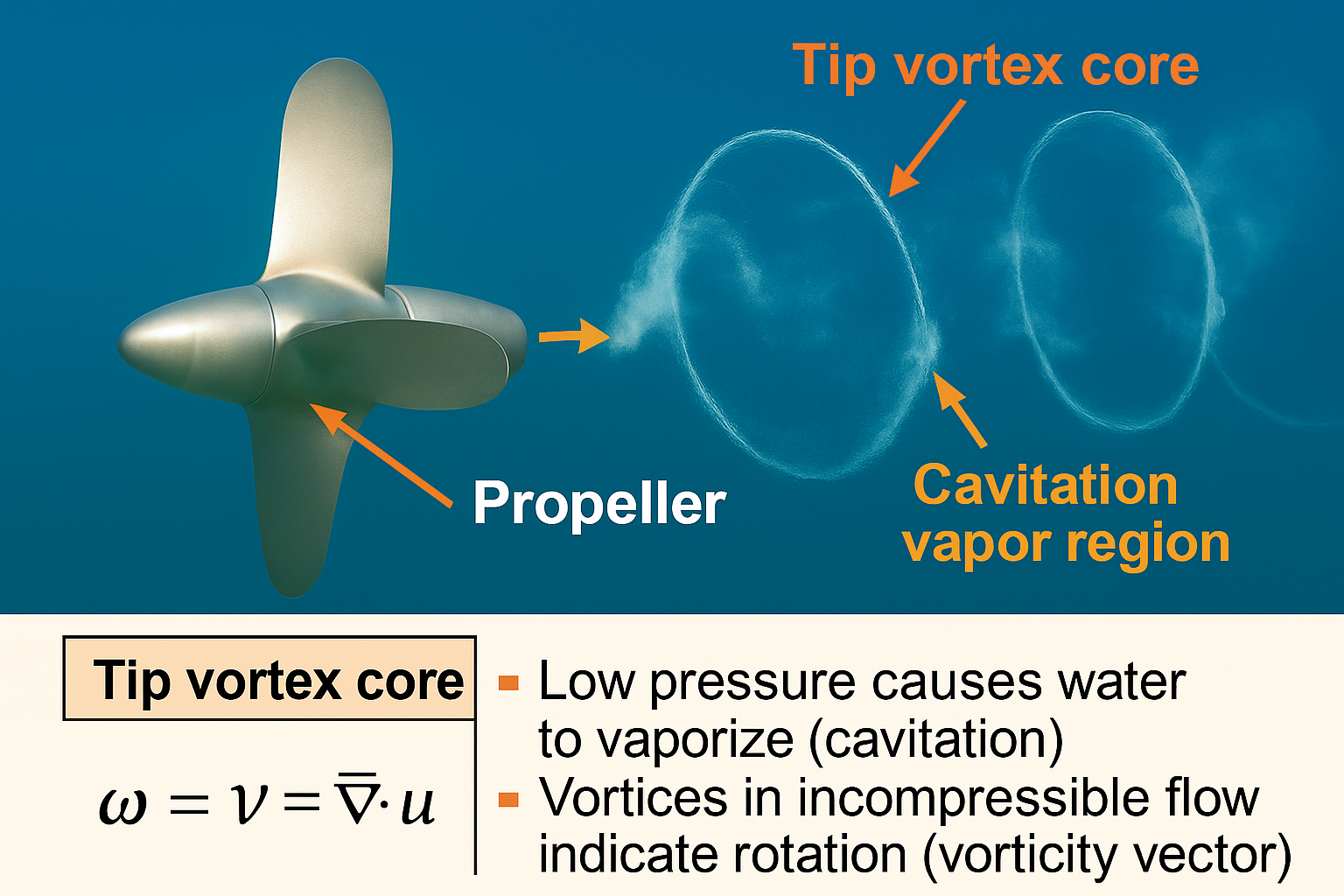
🖼️ Panton — Figure: Water Tunnel Propeller Test
Adapted from: Panton, R. L. Incompressible Flow, 6th ed., Wiley, 2013.
🖼️ Panton — Figure: Coordinate Systems & Stream Function
Adapted from: Panton, R. L. Incompressible Flow, 6th ed., Wiley, 2013.
Pick symmetry-friendly coordinates; use \( \psi \) to enforce \( \nabla\cdot\mathbf{u}=0 \) automatically.
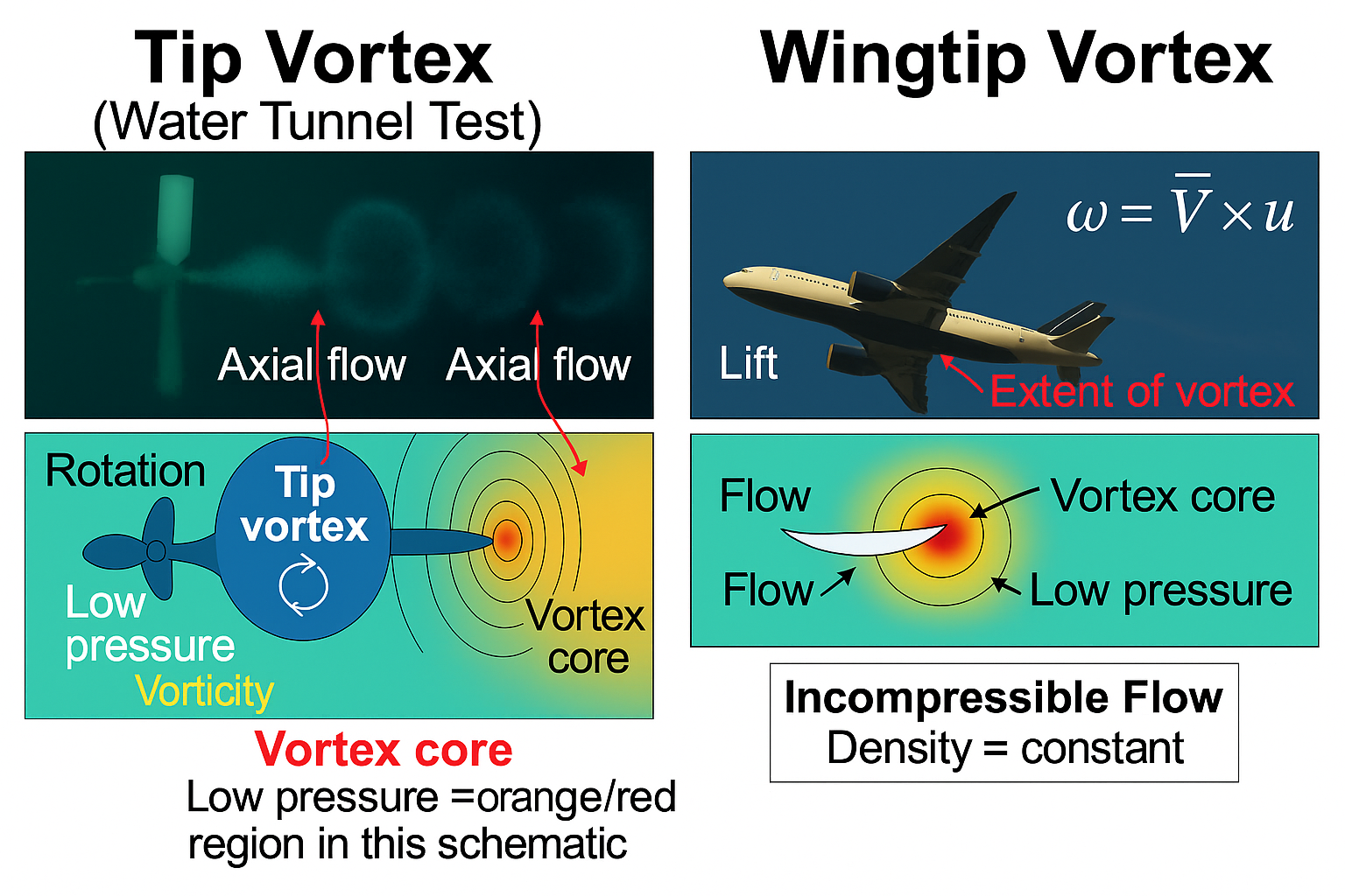
🌀 Extra: Figure 1.1 — Ship Propeller Tip Vortex
🌀 Extra: Figure 1.2 — Aircraft Wingtip Vortex
ℹ️ Context — Why Panton shows these
- Visual hooks for vorticity & circulation before equations.
- Parallels across water/air flows; prepares for BL and potential-flow topics.
Panton, Chapter 1 — Study Guide (1.1–1.6)
Quick Summary What makes a fluid, and when gases act “incompressible” ›
Big picture
A fluid cannot sustain static shear—it keeps deforming. Liquids are nearly incompressible; gases are compressible, but at low Mach many gas flows behave like incompressible.
Use it
If density changes are tiny and \(M=U/c\lesssim 0.3\), model as incompressible even in air.
Full Notes Practical contrasts & rule of thumb ›
Liquids
Nearly fixed volume; surface tension matters; weak compressibility.
Gases
Fill container; \(p\leftrightarrow\rho\) tightly coupled; shocks/waves possible at higher Mach.
Thumb rule
“Incompressible” is usually fine if \( \Delta\rho/\rho\ll 1 \) and \( M\lesssim 0.3 \).
Quick Summary Fields are limits over shrinking volumes ›
Definition idea
- Density \(\rho(\mathbf{x})=\lim_{V\to0}\frac{\sum m_i}{V}\)
- Velocity \(\mathbf{v}(\mathbf{x})=\lim_{V\to0}\frac{\sum m_i\mathbf{v}_i}{\sum m_i}\)
Shrink \(V\) while still \(\gg\) molecular scales and \(\ll\) flow scales → “plateau” values.
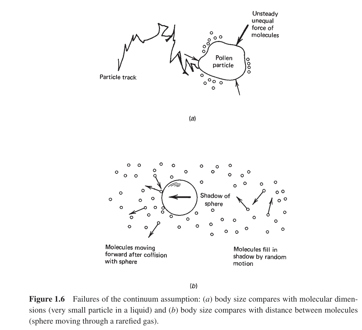
Fails when
Mean free path or particle size \(\sim\) geometry (Kn not small) → rarefied gas, microflows, Brownian/colloids.
Full Notes Plateau picture ›
As \(V\) shrinks from large to small, averages settle (plateau). Past ~molecular scales, noise explodes—work on the plateau.
Quick Summary FR / MR / VR / AR regions & Galilean invariance ›
Region types
- FR Fixed in space (fluid crosses the boundary).
- MR Material region; boundary moves with fluid (no crossing).
- VR Rigid motion with constant volume.
- AR Anything useful (hybrids / analysis-friendly shapes).
Physics
Basic laws keep the same form in any inertial (Galilean) frame.
Full Notes Examples & checks ›
- Blower in lab frame → FR.
- Rising bubble skin → MR (surface speed = local fluid speed).
- Rocket shell following COM with fixed volume → VR.
Quick Summary Clean definitions + split total KE into bulk + random ›
Definitions
- Density \( \rho=\lim_{V\to0}\frac{\sum m_i}{V} \)
- Mass-avg velocity \( \mathbf{v}=\lim_{V\to0}\frac{\sum m_i\mathbf{v}_i}{\sum m_i} \)
- Random velocity \( \mathbf{v}'_i=\mathbf{v}_i-\mathbf{v} \)
- KE split \( \sum \tfrac12 m_i \mathbf{v}_i^2=\sum \tfrac12 m_i \mathbf{v}'^{\,2}_i+\tfrac12\,\mathbf{v}^2 \sum m_i \)
Symbols
Why it holds
Let \( \mathbf{v}_i=\mathbf{v}+\mathbf{v}'_i \). The cross term vanishes since \( \sum m_i\mathbf{v}'_i=\mathbf{0} \).
Quick check
Prove \( \sum m_i\mathbf{v}'_i=\mathbf{0} \) from the definition of \( \mathbf{v} \).
Key ideas
- Internal energy includes random translation, rotation, vibration, potentials.
- Molar-avg equals mass-avg only for uniform composition.
Example
Binary gas with diffusion: species speeds differ from \( \mathbf{v} \) → diffusive fluxes even if the bulk is at rest.
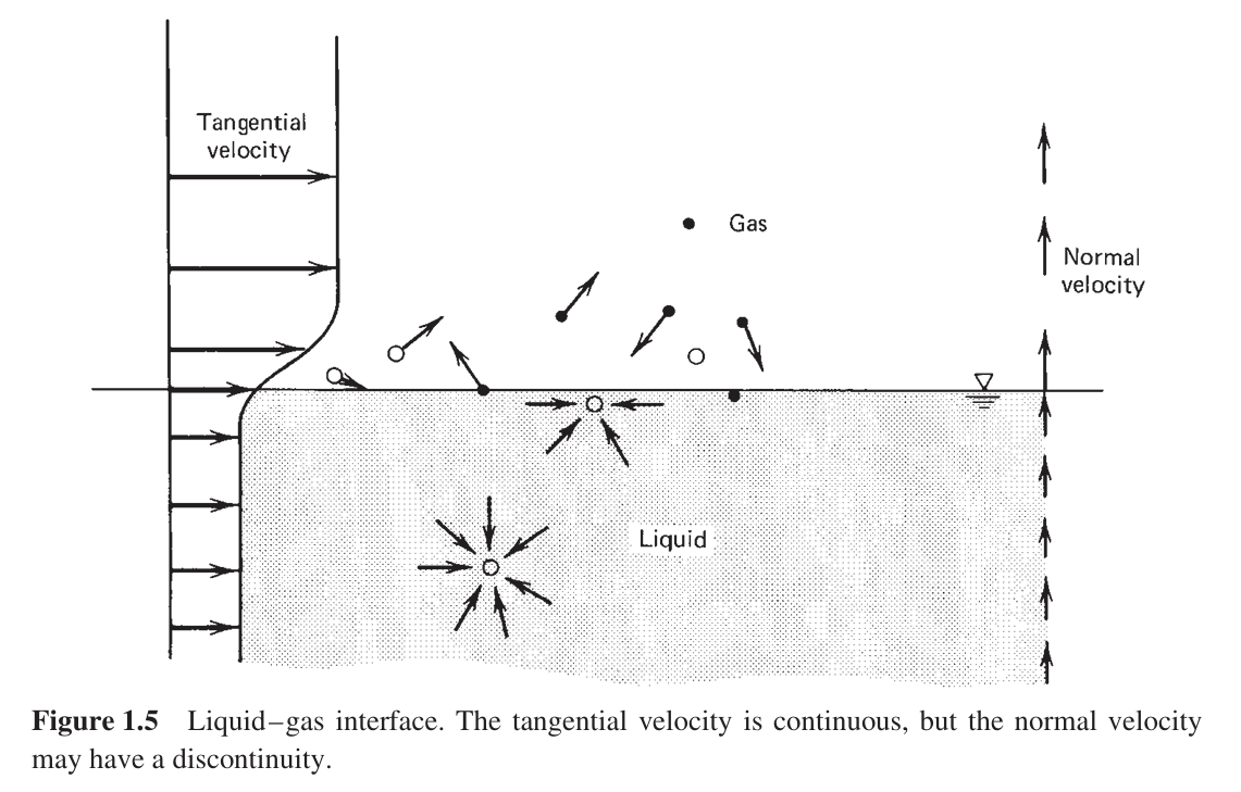
Quick Summary Simple interface model that works most of the time ›
Model
Zero-thickness interface; \( \rho \) may jump; tangential \( \mathbf{v} \) and \( T \) continuous; normal velocity \( v_n \) may jump with mass transfer.
Mass-flux match
\( \rho_\ell v_{n,\ell} = \rho_v v_{n,v} \).
Full Notes No-slip & caveats ›
Key ideas
No-slip tangentially in most cases → same tangential \( \mathbf{v} \) on both sides. With mass transfer, differing normal velocities expected because \( \rho \) differs.
Watch out
Surface tension/surfactants/Marangoni can alter balances—this is the simple model.
Figure 1.5 Liquid–gas interface — what’s continuous, what can jump ›
Quick Summary When continuum breaks & what to use instead ›
Breaks when
Body scale \(L\) \(\sim\) molecular size or mean free path \( \lambda \). Knudsen \( \mathrm{Kn}=\lambda/L \) not small.
Then use
Kinetic/DSMC for gases; stochastic/colloidal models for liquids; slip models in microflows.
Full Notes Practical checks ›
- Air at STP: \( \lambda \approx 0.1\,\mu\text{m} \). If \( L \gg 10\lambda \), continuum is usually safe.
- Incompressible gas flows: typically \( M\lesssim 0.3 \) and small \( \Delta \rho/\rho \).
Figure 1.6 Failures of the Continuum Assumption ›